It’s been quite a while without writing anything. Today, we are going to introduce PyFlux for time seriers analysis. Cannonical models are to be directly adopted from PyFlux Documents and tested in this blog.
Get Started
Copy and paste that piece of code from PyFlux Documents with trivial modifications as follows:
import pandas as pd import numpy as np from pandas_datareader.data import DataReader from datetime import datetime import pyflux as pf import matplotlib.pyplot as plt
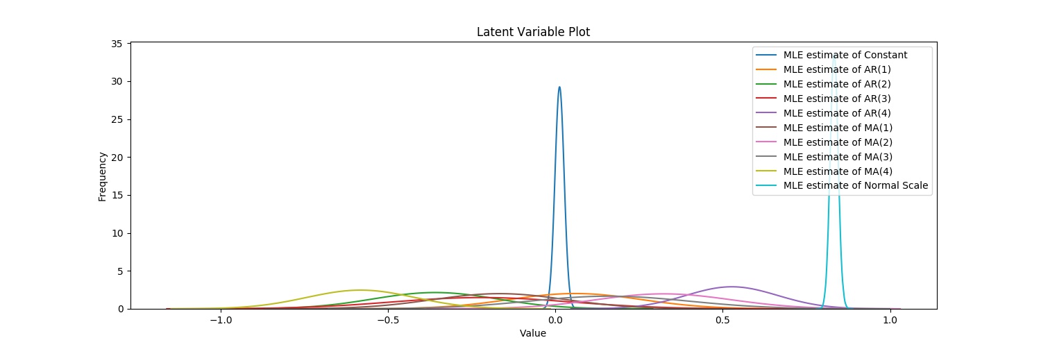
Index    Latent Variable           Prior           Prior Hyperparameters     V.I. Dist  Transform
======== ========================= =============== ========================= ========== ==========
0        Constant                  Normal          mu0: 0, sigma0: 3         Normal     None
1        AR(1)                     Normal          mu0: 0, sigma0: 0.5       Normal     None
2        AR(2)                     Normal          mu0: 0, sigma0: 0.5       Normal     None
3        AR(3)                     Normal          mu0: 0, sigma0: 0.5       Normal     None
4        AR(4)                     Normal          mu0: 0, sigma0: 0.5       Normal     None
5        MA(1)                     Normal          mu0: 0, sigma0: 0.5       Normal     None
6        MA(2)                     Normal          mu0: 0, sigma0: 0.5       Normal     None
7        MA(3)                     Normal          mu0: 0, sigma0: 0.5       Normal     None
8        MA(4)                     Normal          mu0: 0, sigma0: 0.5       Normal     None
9        Normal Scale              Flat            n/a (non-informative)     Normal     exp
~/.local/lib/python3.6/site-packages/numdifftools/limits.py:126: UserWarning: All-NaN slice encountered warnings.warn(str(msg)) Acceptance rate of Metropolis-Hastings is 0.000125 Acceptance rate of Metropolis-Hastings is 0.00075 Acceptance rate of Metropolis-Hastings is 0.105525 Acceptance rate of Metropolis-Hastings is 0.13335 Acceptance rate of Metropolis-Hastings is 0.1907 Acceptance rate of Metropolis-Hastings is 0.232 Acceptance rate of Metropolis-Hastings is 0.299
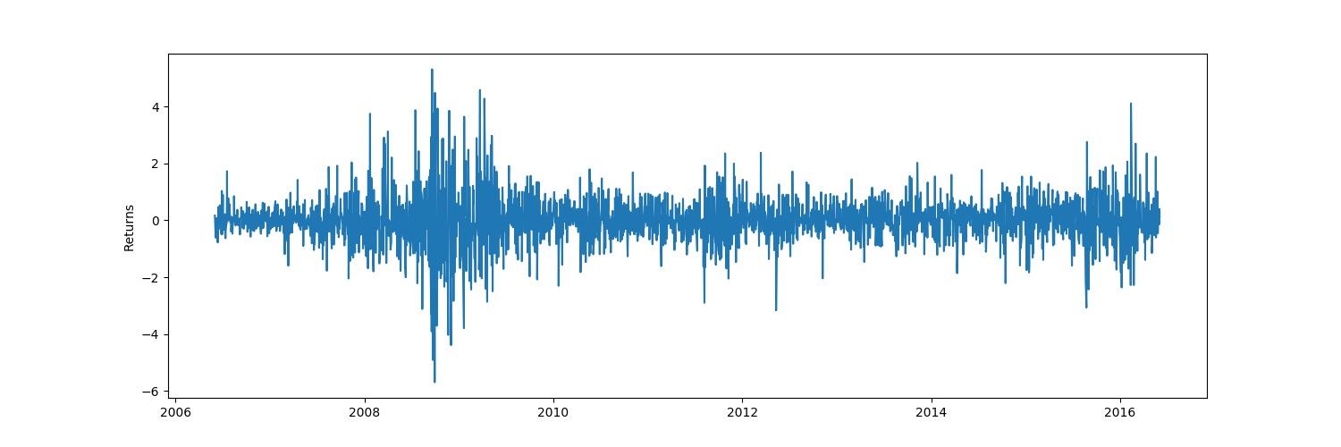
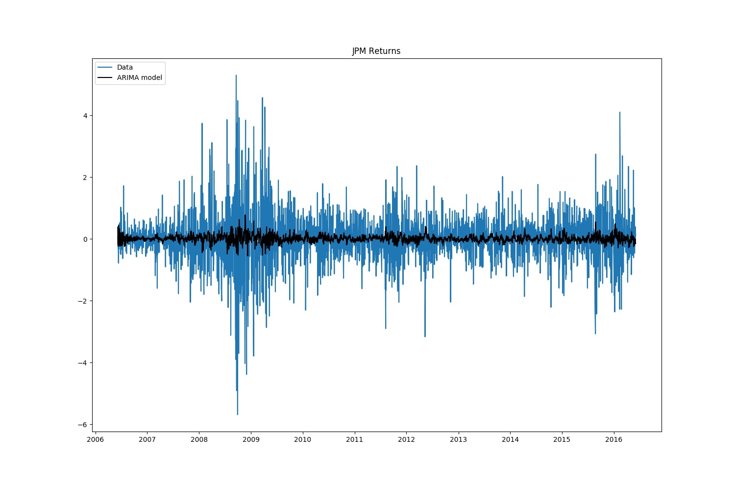
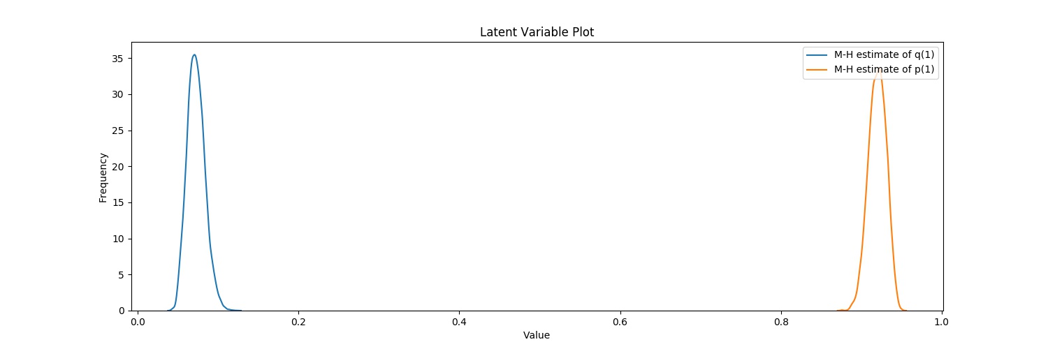
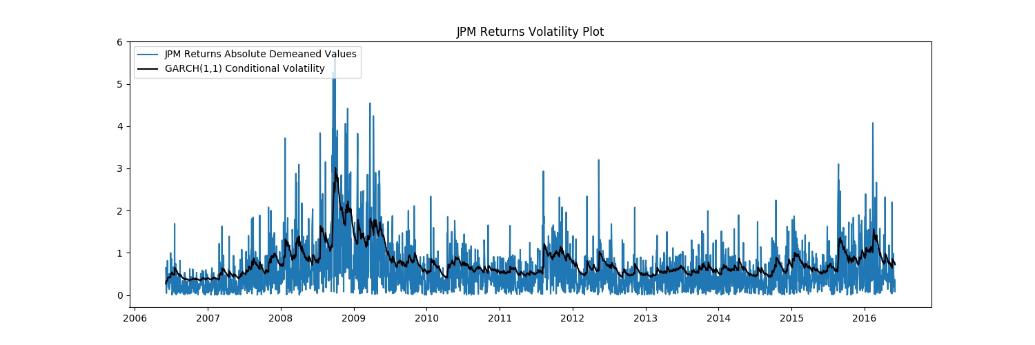
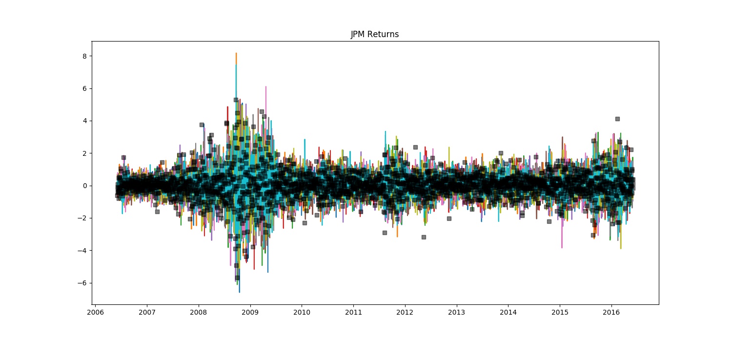
Tuning complete! Now sampling. Acceptance rate of Metropolis-Hastings is 0.36655 GARCH(1,1) ======================================================= ================================================== Dependent Variable: JPM Returns Method: Metropolis Hastings Start Date: 2006-06-05 00:00:00 Unnormalized Log Posterior: -2671.5492 End Date: 2016-06-02 00:00:00 AIC: 5351.717896880396 Number of observations: 2517 BIC: 5375.041188860938 ========================================================================================================== Latent Variable Median Mean 95% Credibility Interval ======================================== ================== ================== ========================= Vol Constant 0.0059 0.0057 (0.004 | 0.0076) q(1) 0.0721 0.0728 (0.0556 | 0.0921) p(1) 0.9202 0.9199 (0.9013 | 0.9373) Returns Constant 0.0311 0.0311 (0.0109 | 0.0511) ==========================================================================================================