Finally, I’ve got some time to write something about PyTorch, a popular deep learning tool. We suppose you have had fundamental understanding of Anaconda Python, created Anaconda virtual environment (in my case, it’s named condaenv), and had PyTorch installed successfully under this Anaconda virtual environment condaenv.
Since I’m using Visual Studio Code to test my Python code (of course, you can use whichever coding tool you like), I suppose you’ve already had your own coding tool configured. Now, you are ready to go!
In my case, I’m giving a tutorial, instead of coding by myself. Therefore, Jupyter Notebook is selected as my presentation tool. So, I’ll demonstrate everything both in .py files, as well as .ipynb files. All codes can be found at Longer Vision PyTorch_Examples. However, ONLY Jupyter Notebook presentation is given in my blogs. Therefore, I suppose you’ve already successfully installed Jupyter Notebook, as well as any other required packages under your Anaconda virtual environment condaenv.
Now, let’s pop up Jupyter Notebook server.
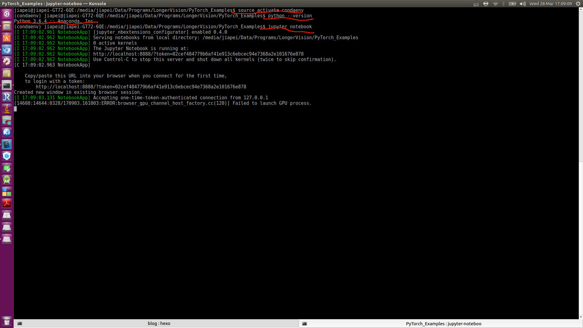
Clearly, Anaconda comes with the NEWEST version. So far, it is Python 3.6.4.
PART A: Hello PyTorch
Our very FIRST test code is of only 6 lines including an empty line:
After popping up Jupyter Notebook server, and click Run, you will see this view:
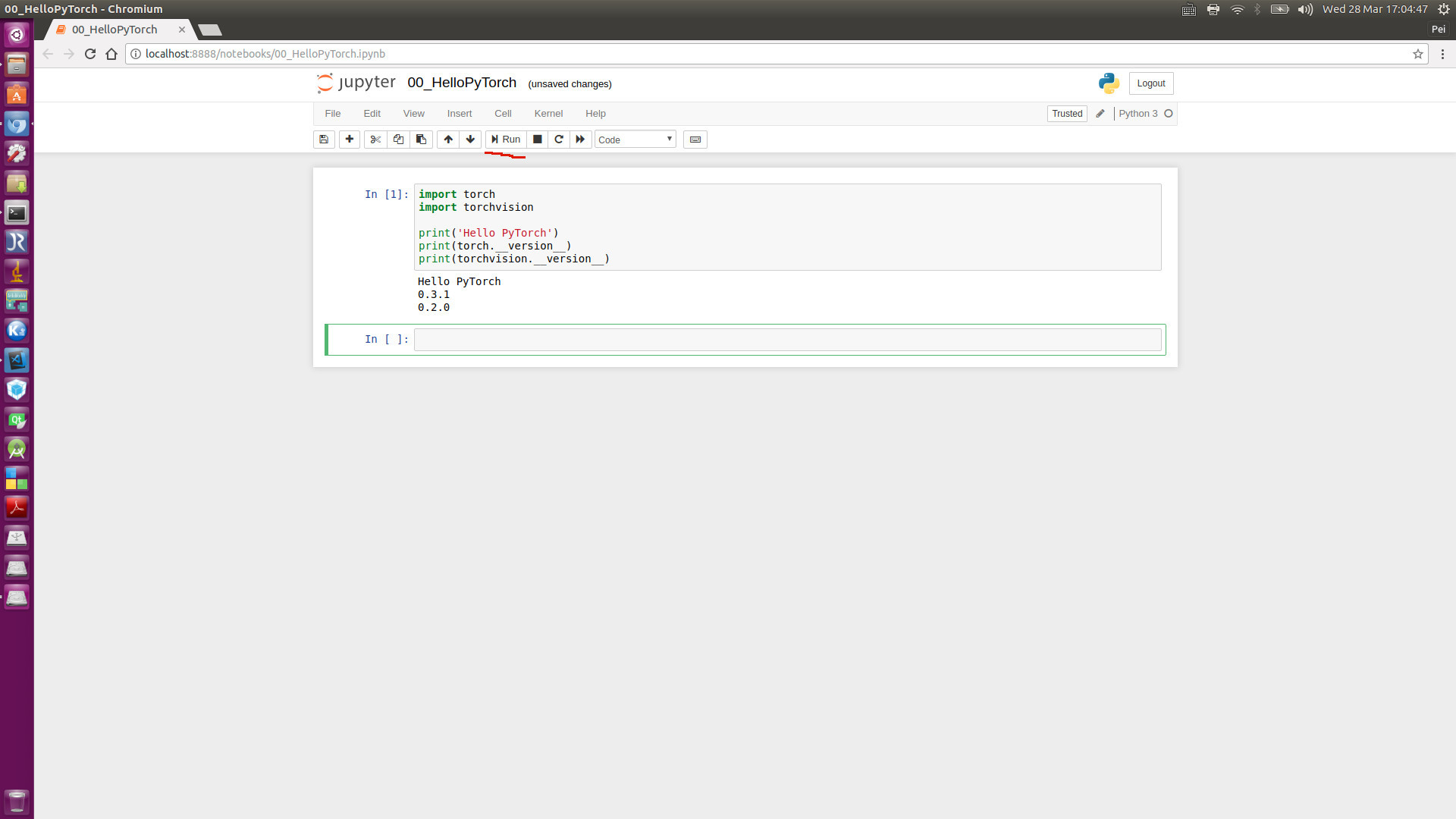
Clearly, the current torch is of version 0.3.1, and torchvision is of version 0.2.0.
PART B: Convolutional Neural Network in PyTorch
1. General Concepts
1) Online Resource
We are NOT going to discuss the background details of Convolutional Neural Network. A lot online frameworks/courses are available for you to catch up:
Several fabulous blogs are strongly recommended, including:
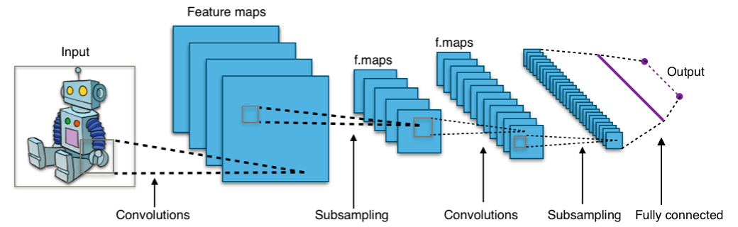
2) Architecture
One picture for all (cited from Convolutional Neural Network )
3) Back Propagation (BP)
The ONLY concept in CNN we want to emphasize here is Back Propagation, which has been widely used in traditional neural networks, which takes the solution similar to the final Fully Connected Layer of CNN. You are welcome to get some more details from https://brilliant.org/wiki/backpropagation/.
Pre-defined Variables
Training Database
- $X={(\vec{x_1},\vec{y_1}),(\vec{x_2},\vec{y_2}),…,(\vec{x_N},\vec{y_N})}$: the training dataset $X$ is composed of $N$ pairs of training samples, where $(\vec{x_i},\vec{y_i}),1 \le i \le N$
- $(\vec{x_i},\vec{y_i}),1 \le i \le N$: the $i$th training sample pair
- $\vec{x_i}$: the $i$th input vector (can be an original image, can also be a vector of extracted features, etc.)
- $\vec{y_i}$: the $i$th desired output vector (can be a one-hot vector, can also be a scalar, which is a 1-element vector)
- $\hat{\vec{y_i} }$: the $i$th output vector from the nerual network by using the $i$th input vector $\vec{x_i}$
- $N$: size of dataset, namely, how many training samples
- $w_{ij}^k$: in the neural network’s architecture, at level $k$, the weight of the node connecting the $i$th input and the $j$th output
- $\theta$: a generalized denotion for any parameter inside the neural networks, which can be looked on as any element from a set of $w_{ij}^k$.
Evaluation Function
- Mean squared error (MSE): $$E(X, \theta) = \frac{1}{2N} \sum_{i=1}^N \left(||\hat{\vec{y_i} } - \vec{y_i}||\right)^2$$
- Cross entropy: $$E(X, prob) = - \frac{1}{N} \sum_{i=1}^N log_2\left({prob(\vec{y_i})}\right)$$
Particularly, for binary classification, logistic regression is often adopted. A logistic function is defined as:
$$f(x)=\frac{1}{(1+e^{-x})}$$
In such a case, the loss function can easily be deducted as:
$$E(X,W) = - \frac{1}{N} \sum_{i=1}^N [y_i log({\hat{y_i} })+(1-y_i)log(1-\hat{y_i})]$$
where
$$y_i=0/1$$
$$\hat{y_i} \equiv g(\vec{w} \cdot \vec{x_i}) = \frac{1}{(1+e^{-\vec{w} \cdot \vec{x_i} })}$$
Some PyTorch explaination can be found at torch.nn.CrossEntropyLoss.
BP Deduction Conclusions
Only MSE is considered here (Please refer to https://brilliant.org/wiki/backpropagation/):
$$
\frac {\partial {E(X,\theta)} } {\partial w_{ij}^k} = \frac {1}{N} \sum_{d=1}^N \frac {\partial}{\partial w_{ij}^k} \Big( {\frac{1}{2} (\vec{y_d}-y_d)^2 } \Big) = \frac{1}{N} \sum_{d=1}^N {\frac{\partial E_d}{\partial w_{ij}^k} }
$$
The updating weights is also determined as:
$$
\Delta w_{ij}^k = - \alpha \frac {\partial {E(X,\theta)} } {\partial w_{ij}^k}
$$